Deep Convolutional Auto Encoders - Part 1
Reimplementing DCAE to encode agent swarm flight


- Introduction
- Details
- Data Noramlisation and preperation
- Define the encoder and decoder
- Training
- Conclusion
Introduction
My aim is to try and encode a simulated swarm into a lower dimentional representation so I can identify interesting parameters with which to map into a sound generating system.
My initial research into reducing complex time-series data lead me to a paper by Ali et al
They use convolutional layers in an auto encoder to do dimension reduction on various time series data.
This seemed like a good place to start, so initially I am just documenting my attempt to recreate their research, using a single agents coordinates in 3d space to match the shape of their model.
Details
Their approach uses 1D Convolution and the data split into interleaved sliding windows of data:
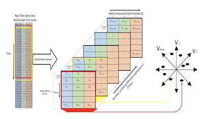
They used a 60 frame window and 3 readings from accelerometers resulting in a 60x3 shape input image.
As a test of their approach I used a single agents movement data to match the original model specifications.
Data is captured from a separate flocking simulation (source available on my github soon) of 300 agents over approximately 30 seconds.
using Flux, CSV, DataFrames, MLDataPattern, CUDA, Plots, WebIO;
plotly()
df = DataFrame(CSV.File("$(datadir())/exp_raw/data.csv"; types=Float32))
df = df[:,1:3]

plot(df[:,1],df[:,2], df[:,3])
We can treat this 3D data as 3 separate 1D data points, matching the original TimeCluster data shape
plot(df[:,1], label="x")
plot!(df[:,2], label="y")
plot!(df[:,3], label="z")
function normalise(M)
    min = minimum(minimum(eachcol(M)))
    max = maximum(maximum(eachcol(M)))
    return (M .- min) ./ (max - min)
end

normalised = Array(df) |> normalise

window_size = 60

data = slidingwindow(normalised',window_size,stride=1);
function create_ae()
    # Define the encoder and decoder networks
  encoder = Chain(
  # 60x3xb
    Conv((10,), 3 => 64, relu; pad = SamePad()),
    MaxPool((2,)),
    # 30x64xb
    Conv((5,), 64 => 32, relu; pad = SamePad()),
    MaxPool((2,)),
    # 15x32xb
    Conv((5,), 32 => 12, relu; pad = SamePad()),
    MaxPool((3,)),
    # 5x12xb
    Flux.flatten,
    Dense(window_size,window_size)
    )
  decoder = Chain(
    # input 60
    (x -> reshape(x, (floor(Int, (window_size / 12)),12,:))),
    # 5x12xb
    ConvTranspose((5,), 12 => 32, relu; pad = SamePad()),
    Upsample((3,)),
    # 15x32xb
    ConvTranspose((5,), 32 => 64, relu; pad = SamePad()),
    Upsample((2,)),
    # 30x64xb
    ConvTranspose((10,), 64 => 3, relu; pad = SamePad()),
    Upsample((2,)),
    # 60x3xb
  )
  return Chain(encoder, decoder)
 end
function train_model!(model, data, opt; epochs=20, bs=16, dev=Flux.gpu)
    model = model |> dev
    ps = params(model)
    t = shuffleobs(data)
    local l
    losses = Vector{Float64}()
    for e in 1:epochs
        for x in eachbatch(t, size=bs)
            # bs[(3, 60)]
            x  = cat(x..., dims=3)
            # bs x 3 x 60
            x  = permutedims(x, [2,1,3])
            # 60 x 3 x bs
            gs = gradient(ps) do
                l = loss(model(x),x)
            end
            Flux.update!(opt, ps, gs)
        end
        l = round(l;digits=6)
        push!(losses, l)
        println("Epoch $e/$epochs - train loss: $l")
    end
    model = model |> cpu;
    losses
 end
loss(x,y) = Flux.Losses.mse(x, y)
opt       = Flux.Optimise.ADAM(0.00005)
epochs    = 100
model     = create_ae()
losses_01 = train_model!(model, data, opt; epochs=epochs);
plot(losses_01, label="")
xlabel!("Epochs")
ylabel!("Mean Squared Error")
Lets see how well it's able to reconstruct a random segment of the data
input = rand(data)'
plot(input[:,1],input[:, 2], input[:,3], label="original")

# Plot the reconstructed data in red
output = model(Flux.unsqueeze(input, 3))
plot!(output[:,1], output[:, 2], output[:,3], label="reconstructed")
@info "loss:" loss(input, output)